Computer Simulations That Teach Themselves To Walk.

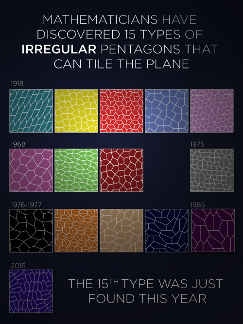
Big math news! It’s been thirty years since mathematicians last found a convex pentagon that could “tile the plane.” The latest discovery (by Jennifer McLoud-Mann, Casey Mann, and David Von Derau) was published earlier this month. Full story.

Fibonacci Sculptures - Part II

These are 3-D printed sculptures designed to animate when spun under a strobe light. The placement of the appendages is determined by the same method nature uses in pinecones and sunflowers. The rotation speed is synchronized to the strobe so that one flash occurs every time the sculpture turns 137.5º—the golden angle. If you count the number of spirals on any of these sculptures you will find that they are always Fibonacci numbers.

© John Edmark

Everyone who reblogs this will get a pick-me-up in their ask box.

Every. Single. One. Of. You.

Permutations

Figuring out how to arrange things is pretty important.

Like, if we have the letters {A,B,C}, the six ways to arrange them are: ABC ACB BAC BCA CAB CBA

And we can say more interesting things about them (e.g. Combinatorics) another great extension is when we get dynamic

Like, if we go from ABC to ACB, and back…

We can abstract away from needing to use individual letters, and say these are both “switching the 2nd and 3rd elements,” and it is the same thing both times.

Each of these switches can be more complicated than that, like going from ABCDE to EDACB is really just 1->3->4->2->5->1, and we can do it 5 times and cycle back to the start

We can also have two switches happening at once, like 1->2->3->1 and 4->5->4, and this cycles through 6 times to get to the start.

Then, let’s extend this a bit further.

First, let’s first get a better notation, and use (1 2 3) for what I called 1->2->3->1 before.

Let’s show how we can turn these permutations into a group.

Then, let’s say the identity is just keeping things the same, and call it id.

And, this repeating thing can be extended into making the group combiner: doing one permutation and then the other. For various historical reasons, the combination of permutation A and then permutation B is B·A.

This is closed, because permuting all the things and then permuting them again still keeps 1 of all the elements in an order.

Inverses exist, because you just need to put everything from the new position into the old position to reverse it.

Associativity will be left as an exercise to the reader (read: I don’t want to prove it)

Regarding Fractals and Non-Integral Dimensionality

Alright, I know it’s past midnight (at least it is where I am), but let’s talk about fractal geometry.

Fractals

If you don’t know what fractals are, they’re essentially just any shape that gets rougher (or has more detail) as you zoom in, rather than getting smoother. Non-fractals include easy geometric shapes like squares, circles, and triangles, while fractals include more complex or natural shapes like the coast of Great Britain, Sierpinski’s Triangle, or a Koch Snowflake.

Fractals, in turn, can be broken down further. Some fractals are the product of an iterative process and repeat smaller versions of themselves throughout them. Others are more natural and just happen to be more jagged.

Fractals and Non-Integral Dimensionality

Now that we’ve gotten the actual explanation of what fractals are out of the way, let’s talk about their most interesting property: non-integral dimensionality. The idea that fractals do not actually have an integral dimension was originally thought up by this guy, Benoit Mandelbrot.

He studied fractals a lot, even finding one of his own: the Mandelbrot Set. The important thing about this guy is that he realized that fractals are interesting when it comes to defining their dimension. Most regular shapes can have their dimension found easily: lines with their finite length but no width or height; squares with their finite length and width but no height; and cubes with their finite length, width, and height. Take note that each dimension has its own measure. The deal with many fractals is that they can’t be measured very easily at all using these terms. Take Sierpinski’s triangle as an example.

Is this shape one- or two-dimensional? Many would say two-dimensional from first glance, but the same shape can be created using a line rather than a triangle.

So now it seems a bit more tricky. Is it one-dimensional since it can be made out of a line, or is it two-dimensional since it can be made out of a triangle? The answer is neither. The problem is that, if we were to treat it like a two-dimensional object, the measure of its dimension (area) would be zero. This is because we’ve technically taken away all of its area by taking out smaller and smaller triangles in every available space. On the other hand, if we were to treat it like a one-dimensional object, the measure of its dimension (length) would be infinity. This is because the line keeps getting longer and longer to stretch around each and every hole, of which there are an infinite number. So now we run into a problem: if it’s neither one- nor two-dimensional, then what is its dimensionality? To find out, we can use non-fractals

Measuring Integral Dimensions and Applying to Fractals

Let’s start with a one-dimensional line. The measure for a one-dimensional object is length. If we were to scale the line down by one-half, what is the fraction of the new length compared to the original length?

The new length of each line is one-half the original length.

Now let’s try the same thing for squares. The measure for a two-dimensional object is area. If we were to scale down a square by one-half (that is to say, if we were to divide the square’s length in half and divide its width in half), what is the fraction of the new area compared to the original area?

The new area of each square is one-quarter the original area.

If we were to try the same with cubes, the volume of each new cube would be one-eighth the original volume of a cube. These fractions provide us with a pattern we can work with.

In one dimension, the new length (one-half) is equal to the scaling factor (one-half) put to the first power (given by it being one-dimensional).

In two dimensions, the new area (one-quarter) is equal to the scaling factor (one-half) put to the second power (given by it being two-dimensional).

In three dimensions, the same pattern follows suit, in which the new volume (one-eighth) is equivalent to the scaling factor (one-half) put to the third power.

We can infer from this trend that the dimension of an object could be (not is) defined as the exponent fixed to the scaling factor of an object that determines the new measure of the object. To put it in mathematical terms:

Examples of this equation would include the one-dimensional line, the two-dimensional square, and the three-dimensional cube:

½ = ½^1

¼ = ½^2

1/8 = ½^3

Now this equation can be used to define the dimensionality of a given fractal. Let’s try Sierpinski’s Triangle again.

Here we can see that the triangle as a whole is made from three smaller versions of itself, each of which is scaled down by half of the original (this is proven by each side of the smaller triangles being half the length of the side of the whole triangle). So now we can just plug in the numbers to our equation and leave the dimension slot blank.

1/3 = ½^D

To solve for D, we need to know what power ½ must be put to in order to get 1/3. To do this, we can use logarithms (quick note: in this case, we can replace ½ with 2 and 1/3 with 3).

log_2(3) = roughly 1.585

So we can conclude that Sierpinski’s triangle is 1.585-dimensional. Now we can repeat this process with many other fractals. For example, this Sierpinski-esque square:

It’s made up of eight smaller versions of itself, each of which is scaled down by one-third. Plugging this into the equation, we get

1/8 = 1/3^D

log_3(8) = roughly 1.893

So we can conclude that this square fractal is 1.893-dimensional.

We can do this on this cubic version of it, too:

This cube is made up of 20 smaller versions of itself, each of which is scaled down by 1/3.

1/20 = 1/3^D

log_3(20) = roughly 2.727

So we can conclude that this fractal is 2.727-dimensional.

We Need Your Help to Find STEVE

Glowing in mostly purple and green colors, a newly discovered celestial phenomenon is sparking the interest of scientists, photographers and astronauts. The display was initially discovered by a group of citizen scientists who took pictures of the unusual lights and playfully named them “Steve.”

When scientists got involved and learned more about these purples and greens, they wanted to keep the name as an homage to its initial name and citizen science discoverers. Now it is STEVE, short for Strong Thermal Emission Velocity Enhancement.

Credit: ©Megan Hoffman

STEVE occurs closer to the equator than where most aurora appear – for example, Southern Canada – in areas known as the sub-auroral zone. Because auroral activity in this zone is not well researched, studying STEVE will help scientists learn about the chemical and physical processes going on there. This helps us paint a better picture of how Earth’s magnetic fields function and interact with charged particles in space. Ultimately, scientists can use this information to better understand the space weather near Earth, which can interfere with satellites and communications signals.

Want to become a citizen scientist and help us learn more about STEVE? You can submit your photos to a citizen science project called Aurorasaurus, funded by NASA and the National Science Foundation. Aurorasaurus tracks appearances of auroras – and now STEVE – around the world through reports and photographs submitted via a mobile app and on aurorasaurus.org.

Here are six tips from what we have learned so far to help you spot STEVE:

1. STEVE is a very narrow arc, aligned East-West, and extends for hundreds or thousands of miles.

Credit: ©Megan Hoffman 

2. STEVE mostly emits light in purple hues. Sometimes the phenomenon is accompanied by a short-lived, rapidly evolving green picket fence structure (example below).

Credit: ©Megan Hoffman 

3. STEVE can last 20 minutes to an hour.

4. STEVE appears closer to the equator than where normal – often green – auroras appear. It appears approximately 5-10° further south in the Northern hemisphere. This means it could appear overhead at latitudes similar to Calgary, Canada. The phenomenon has been reported from the United Kingdom, Canada, Alaska, northern US states, and New Zealand.

5. STEVE has only been spotted so far in the presence of an aurora (but auroras often occur without STEVE). Scientists are investigating to learn more about how the two phenomena are connected. 

6. STEVE may only appear in certain seasons. It was not observed from October 2016 to February 2017. It also was not seen from October 2017 to February 2018.

Credit: ©Megan Hoffman 

STEVE (and aurora) sightings can be reported at www.aurorasaurus.org or with the Aurorasaurus free mobile apps on Android and iOS. Anyone can sign up, receive alerts, and submit reports for free.

Make sure to follow us on Tumblr for your regular dose of space: http://nasa.tumblr.com.

Planetary Frequencies.

Geometry and Divnity

Omnipresence

The Point

Divinity is present in every aspect of natural order and causality dimensions. It is part of the material world through various holistic and messianic incarnations, being at the same time a component of human thought and action. This kind of omnipresence is logical possible through the classical definition of a geometrical point, that is part of the entire space but does not occupy any of it.

Trinity

The Borromean Rings

While distinct and at the same time considered to be one in all else, the Three Divine Persons are sometimes represented by the Borromean Rings: no two of the three rings are linked with each other,but nonetheless all three are linked.

Divinity

Harmonic Proportion

The harmonic state of an element is associated with beauty, given by the equilibrium of its components. Nature is being perceived as beautiful, and its creator as good - inevitable and inherently in harmony with its creation.

(Source: Adam Plouff)